앞서 공부했던, 'Attention is All You Need'와 GPT-1논문을 기반으로 한 간단한 프로젝트를 구현해보자.
2025.07.26 - [paper review] - Attention Is All You Need Review
Attention Is All You Need Review
"Attention Is All You Need" paper는 현대 인공지능의 패러다임 자체를 바꿔버린 역사적인 논문이다. '시대를 바꾼 논문' 이라는 표현이 과장이 아닐정도로, 이 논문 직후에 많은 곳에서 'self-attention' 방
wm07070.tistory.com
Improving Language Understanding by Generative Pre-Training(GPT -1) Review
https://cdn.openai.com/research-covers/language-unsupervised/language_understanding_paper.pdfOpenAI에서 만든 GPT(Generative Pre-trained Transformer)의 시초가 되는 논문으로, GPT-1에 해당한다. 이후, GPT1 -> GPT-2 → GPT-3 → GPT-4으
wm07070.tistory.com
Self-Attention 구조를 가진 Decoder-Only Transformer(GPT 1)을 구현할 것이고, 다음 영상을 참고하였다.
https://youtu.be/kCc8FmEb1nY?si=MIHI2XejrAOde7hl
우선, 모델의 코드를 알아보기 전에, 이론적인 내용부터 복습하고 넘어가자.
Transformer
Transformer는 RNN 없이 시퀀스를 처리하기 위해 제안된 모델이다. 핵심은 Self-Attention을 이용해 입력 시퀀스의 모든 위치가 서로를 참조할 수 있게 하는 것.
- 입력: 토큰(문자, 단어 등)을 숫자로 변환한 시퀀스
- 출력: 번역, 문장 생성, 다음 단어 예측 등
구조적으로는 **인코더(Encoder)**와 **디코더(Decoder)**로 나뉘지만, GPT 계열은 디코더만 사용한다. 이번 모델에서도 디코더만 사용. 또한, 복잡한 gpt모델에서는 토큰을 단어 혹은 유의미한 단어구로 설정하지만, 우리는 간단한 모델 구현이 목표이므로, 문자 하나를 토큰 단위로 정했다. 총 65개의 토큰종류가 생기는데, 이는 a~Z와 0~9그리고 다양한 기호(.,!?/..)등을 포함한 것이다.
Self-Attention
Q, K, V 벡터
각 입력 토큰 임베딩에서 세 가지 벡터를 만든다.
- Query (Q): 내가 어떤 정보를 찾고 싶은지
- Key (K): 내가 어떤 정보를 제공할 수 있는지
- Value (V): 실제 전달할 정보
유사도 계산
- QK^T → Query와 Key의 내적
- \frac{1}{\sqrt{d_k}} 로 나눠 스케일링
- Softmax로 가중치 계산
- 가중치 × V를 해서 최종 출력
Multi‑Head Attention
- 여러 head가 서로 다른 서브공간에서 attention을 계산(평행 시점).
- head 출력들을 concat → 선형 투영으로 다시 d_model(n_embd)에 맞춤.
Position (순서) 정보
sequence 내에서 token간의 유의미한 정보를 만들기 위해서는 위치 정보인 position embedding이 필요하다.
- 원 Transformer(Attention Is All You Need): 고정 사인/코사인(sinusoidal)을 사용해서 positional embedding을 정했다.(fixed).
- 반면, 많은 LLM(GPT 계열)에서는 learned positional embedding(학습 O)을 사용한다. 우리 모델도 gpt1을 모방하여, 시간에 걸쳐 최적의 값으로 학습되는 positional embedding을 사용할 것이다.
Transformer Block
self-attention transformer에서는 encoder/decoder에서 residual connection과 layer normalization을 해주었다.
residual connection이란, y = x + F(x) 로, 출력에 입력을 더하는 구조이다.
이러한 구조는 기울기 소실을 막고, 정보를 보존하며, 깊은 모델을 안정적으로 학습하게 만들어 준다.
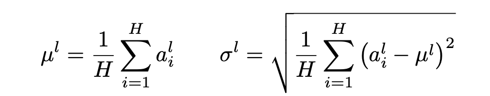
layer normalization은 입력 벡터의 모든 feature 차원(채널)**을 따라 평균과 표준편차를 계산하여 정규화하는 방법으로 다음과 같다.
model에서는 Layer가 깊어질 수록, 행렬 합/곱 연산이 발생하는데, 그 과정에서 기울기가 소실/폭발 할 수 있어서, 정규화를 통해 안정성및 성능을 높여주는 것이다.
- Pre‑LayerNorm + Residual 두 번:
- LN → MHA → Dropout → Residual
- LN → FFN(두 개 Linear + 활성화) → Dropout → Residual
- GPT1 논문에서는 norm을 나중에 해주지만, 최근 gpt계열 모델에서는 pre-norm을 하는 것이 대세임.(아래 figure을 확인하자).

Decoder‑Only vs Encoder‑Decoder
- 원 Transformer는 Encoder + Decoder(번역 등).
- GPT‑1은 Decoder‑Only(마스크드 self‑attention): 순차 생성용.
이제, 자세한 코드 구조를 총 5개의 part로 나누어 알아보자.
0. Hyperparameters
1. Data Handling
2. Batch
3. Multi-Head Attention **
4. Feed Forward
5. GPT Model
6. testing(main)
0. Hyperparameters
# hyperparameters
batch_size = 64 # how many independent sequences will we process in parallel?
block_size = 256 # what is the maximum context length for predictions?
max_iters = 5000
eval_interval = 500
learning_rate = 3e-4
device = 'cuda' if torch.cuda.is_available() else 'cpu'
eval_iters = 200
n_embd = 384
n_head = 6
n_layer = 6
dropout = 0.2
# ------------
전체 코드에서 사용하는 중요한 변수들을 정의하고 가자.
batch_size는 한번에 병렬적으로 학습할 문자의 개수이다.
block_size는 한 문장의 길이를 의미한다. (아래의 BLOCK과는 연관 없음.)
max_iters, eval_interval,eval_iters은 생성할 때 설정해주는 값.
n_embd는 token embedding벡터의 차원(크기)를 의미한다.
ex) 'a'를 embedding하면 길이가 n_embd인 벡터로 바뀐다.
n_head는 multi head의 head 개수이다.
n_layer은 block의 개수이다. (Block은 Multi-Head Self-Attention + Feed Forward + Residual + LayerNorm으로 구성된 Transformer의 한 층)-> 뒤에서 구조를 보면서 다루게 될 것이다.
dropout은 나중에 dropout해주는 비율.(뉴런의 20%가 drop out 되는 것임)
cf**) 초반에 헷갈린 점 정리..
Head VS Block
처음에 multi-head를 하면서 왜 또 block이라는 것을 multi-head를 감싸서, block을 여러번 쌓아서 실행하는지 의문이 들어서 정리를 해보자면,
head안에는 batch_size만큼의 문장이 있어서, 문장들을 독립적으로 학습하게 되고, 한번의 head연산으로는, 문장의 깊은 이해를 할 수 없기 때문에, multi-head 구조로 독립적인 head 학습을 진행하는 것이다. head는 모두 독립적으로 진행되기 때문에, 동시에 병렬적으로 수행되고 그 결과가 마지막에 합쳐지게 되는 것이다. (concat)
ex) 첫번째 head는 vowel 파악, 두번째는 주어/동사 구조 파악.. 등등
반면에, block은 쌓으면서 진행되는 거라, 병렬이 아닌 순차적으로 진행된다.
첫번째 block이 진행되면 그 output이 다음 block의 input으로 사용되는 것이다. 이렇게 깊은 block층을 반복하면 더 고차원적인 패턴으로 발전하게 된다.
1. Data Handling
# wget https://raw.githubusercontent.com/karpathy/char-rnn/master/data/tinyshakespeare/input.txt
with open('input.txt', 'r', encoding='utf-8') as f:
    text = f.read()

# here are all the unique characters that occur in this text
chars = sorted(list(set(text)))
vocab_size = len(chars)
# create a mapping from characters to integers
stoi = { ch:i for i,ch in enumerate(chars) }
itos = { i:ch for i,ch in enumerate(chars) }
encode = lambda s: [stoi[c] for c in s] # encoder: take a string, output a list of integers
decode = lambda l: ''.join([itos[i] for i in l]) # decoder: take a list of integers, output a string

# Train and test splits
data = torch.tensor(encode(text), dtype=torch.long)
n = int(0.9*len(data)) # first 90% will be train, rest val
train_data = data[:n]
val_data = data[n:]
이 모델에서 사용할 데이터는 tinyshakespeare에서 가져온다.
다음은 tinyshakespeare 일부이다.
First Citizen:
Before we proceed any further, hear me speak.

All:
Speak, speak.

First Citizen:
You are all resolved rather to die than to famish?

All:
Resolved. resolved.

First Citizen:
First, you know Caius Marcius is chief enemy to the people.

All:
We know't, we know't.

First Citizen:
Let us kill him, and we'll have corn at our own price.
Is't a verdict?

All:
No more talking on't; let it be done: away, away!

Second Citizen:
One word, good citizens.

First Citizen:
We are accounted poor citizens, the patricians good.
What authority surfeits on would relieve us: if they
would yield us but the superfluity, while it were
wholesome, we might guess they relieved us humanely;
but they think we are too dear: the leanness that
afflicts us, the object of our misery, is as an
inventory to particularise their abundance; our
sufferance is a gain to them Let us revenge this with
our pikes, ere we become rakes: for the gods know I
speak this in hunger for bread, not in thirst for revenge.
chars에는 tinyshakespeare에서 사용하는 모든 character을 list만들고, encode/decode를 통해, 문자 <->숫자 기능을 만들어준다.
data는 tinyshakespeare를 encode한 것들을 사용하는데, 90%는 train data로 나머지 10%는 validation data로 분리해준다.
2. Batch
def get_batch(split):
    # generate a small batch of data of inputs x and targets y
    data = train_data if split == 'train' else val_data
    ix = torch.randint(len(data) - block_size, (batch_size,))
    x = torch.stack([data[i:i+block_size] for i in ix])
    y = torch.stack([data[i+1:i+block_size+1] for i in ix])
    x, y = x.to(device), y.to(device)
    return x, y

@torch.no_grad()
get_batch는 우리가 사용할 batch를 data에서 랜덤하게 가져오기 위해 사용된다.
ix는 각 batch가 시작하는 인덱스로, len(data)-block_size는 문장길이를 고려하기 위해서 설정하였다.
x는 input으로 사용하는 값으로 batch_size X block_size 이다.
y는 i+1을 사용해서, x의 다음 토큰 값을 사용한, 결과값이고, shape은 x와 동일하다.
3. Multi-head Attention
이번 모델에서 가장 핵심이 되는 부분이다.
q*k = v를 구현해야 하고, 각 토큰끼리의 관계도 계산해야된다. 단, 미래의 값을 알 수 없게 masking도 추가해주어야 한다.
class Head(nn.Module):
    """ one head of self-attention """

    def __init__(self, head_size):
        super().__init__()
        self.key = nn.Linear(n_embd, head_size, bias=False)
        self.query = nn.Linear(n_embd, head_size, bias=False)
        self.value = nn.Linear(n_embd, head_size, bias=False)
        self.register_buffer('tril', torch.tril(torch.ones(block_size, block_size)))

        self.dropout = nn.Dropout(dropout)

    def forward(self, x):
        # input of size (batch, time-step, channels)
        # output of size (batch, time-step, head size)
        B,T,C = x.shape
        k = self.key(x)   # (B,T,hs)
        q = self.query(x) # (B,T,hs)
        # compute attention scores ("affinities")
        wei = q @ k.transpose(-2,-1) * k.shape[-1]**-0.5 # (B, T, hs) @ (B, hs, T) -> (B, T, T)
        wei = wei.masked_fill(self.tril[:T, :T] == 0, float('-inf')) # (B, T, T)
        wei = F.softmax(wei, dim=-1) # (B, T, T)
        wei = self.dropout(wei)
        # perform the weighted aggregation of the values
        v = self.value(x) # (B,T,hs)
        out = wei @ v # (B, T, T) @ (B, T, hs) -> (B, T, hs)
        return out
Head에서는 Q, K, V를 만들고, dot-product attention을 수행한다.
torch.tril은 행렬의 대각선 기준 위쪽 삼각형을 0으로 masking해주는 함수인데, 이 값은 parameter가 아니라 buffer에 저장해준다.
wei는 가중치 행렬로, qk^T과 softmax를 해서 확률로 바꿔준 값을 v에 곱해 사용하게 된다.
class MultiHeadAttention(nn.Module):
    """ multiple heads of self-attention in parallel """

    def __init__(self, num_heads, head_size):
        super().__init__()
        self.heads = nn.ModuleList([Head(head_size) for _ in range(num_heads)])
        self.proj = nn.Linear(head_size * num_heads, n_embd)
        self.dropout = nn.Dropout(dropout)

    def forward(self, x):
        out = torch.cat([h(x) for h in self.heads], dim=-1)
        out = self.dropout(self.proj(out))
        return out
MultiHeadAttention은 Head를 num_heads만큼 list에 담아서 사용한다.
각 head들의 결과를 concatenate해주고, head_size*num_heads차원을 n_embd로 바꿔서 (B, T, n_embd)의 형태를 맞춰준다.
4. Feedforward
class FeedFoward(nn.Module):
    """ a simple linear layer followed by a non-linearity """

    def __init__(self, n_embd):
        super().__init__()
        self.net = nn.Sequential(
            nn.Linear(n_embd, 4 * n_embd),
            nn.ReLU(),
            nn.Linear(4 * n_embd, n_embd),
            nn.Dropout(dropout),
        )

    def forward(self, x):
        return self.net(x)
Self Attention이후 실행되는 feedforward 부분이다.
ReLU함수를 non-linear function으로 사용해주었고, 논문에서 ReLU입력차원을 512 에서 2048로 4배로 해준 것처럼, n_embd을 4배로 확장시켜서 대입하고, 결과는 다시 차원을 축소시켜주었다.
이렇게, 비선형 함수의 input을 확장 시켜주면, 표현력이 증가한다. 특히 4배가 가장 효과가 좋았다.(from AIAYN)

5. GPT Model
class Block(nn.Module):
    """ Transformer block: communication followed by computation """

    def __init__(self, n_embd, n_head):
        # n_embd: embedding dimension, n_head: the number of heads we'd like
        super().__init__()
        head_size = n_embd // n_head
        self.sa = MultiHeadAttention(n_head, head_size)
        self.ffwd = FeedFoward(n_embd)
        self.ln1 = nn.LayerNorm(n_embd)
        self.ln2 = nn.LayerNorm(n_embd)

    def forward(self, x):
        x = x + self.sa(self.ln1(x))
        x = x + self.ffwd(self.ln2(x))
        return x
전체 모델부분을 보기전에 Block Class를 확인해보자.
Block은 앞서 말했듯이, SA와 FFN을 포함한다.
head크기는 n_embd // n_head(헤드개수)로 정의하고, n_head개수의 mutliheadattention을 실행한다.
이때, gpt에서 사용한 residual connection + normalization을 사용하는데, 앞서 말했듯이, gpt1논문에서는 normalization을 sa와 ffwd 이후에 하지만, 최신 경향을 반영해서 우리는 pre-norm, 즉 normalization을 먼저 해준다.
x = x+ self.sa(self.ln1(x)) 구조가 residual 구조고, sa안에 self.ln1(x)이 들어간것이 pre-norm 구조이다.
이제 최종적으로 main 모델 구조를 확인해보자. (3개의 part로 나누어서 보자)
class GPTLanguageModel(nn.Module):

    def __init__(self):
        super().__init__()
        # each token directly reads off the logits for the next token from a lookup table
        self.token_embedding_table = nn.Embedding(vocab_size, n_embd)
        self.position_embedding_table = nn.Embedding(block_size, n_embd)
        self.blocks = nn.Sequential(*[Block(n_embd, n_head=n_head) for _ in range(n_layer)])
        self.ln_f = nn.LayerNorm(n_embd) # final layer norm
        self.lm_head = nn.Linear(n_embd, vocab_size)

        # better init, not covered in the original GPT video, but important, will cover in followup video
        self.apply(self._init_weights)

    def _init_weights(self, module):
        if isinstance(module, nn.Linear):
            torch.nn.init.normal_(module.weight, mean=0.0, std=0.02)
            if module.bias is not None:
                torch.nn.init.zeros_(module.bias)
        elif isinstance(module, nn.Embedding):
            torch.nn.init.normal_(module.weight, mean=0.0, std=0.02)
앞 부분은 모델 구조를 설정한다.
token_embedding_table은 lookup table로 vocab_size(65:char종류개수)x n_embd(embedding vec길이)의 크기를 가진다.
처음엔 의미없는 값이지만, 학습이 되면서 유의미한 Lookup table로 변할 것이다.
position_embedding_table은 위치 정보를 가진다.
blocks는 n_layer만큼 Block을 쌓아주는 것으로, 우리는 6개의 block을 사용한다.
self.ln_f = nn.LayerNorm(n_embd) # final layer norm
self.lm_head = nn.Linear(n_embd, vocab_size)
은 마지막에 한번 normalization해주고, 이 word embedding vec을 vocab_size의 실제 단어를 encoding한 vec로 만들어주는 과정이다. 이 lm_head는 softmax를 통해 각 토큰이 다음에 올 확률로 변형될 것이다.
init_weights는 전체 가중치를 초기화해주는 함수이다 .
    def forward(self, idx, targets=None):
        B, T = idx.shape

        # idx and targets are both (B,T) tensor of integers
        tok_emb = self.token_embedding_table(idx) # (B,T,C)
        pos_emb = self.position_embedding_table(torch.arange(T, device=device)) # (T,C)
        # print(tok_emb.shape,pos_emb.shape)
        x = tok_emb + pos_emb # (B,T,C)
        x = self.blocks(x) # (B,T,C)
        x = self.ln_f(x) # (B,T,C)
        logits = self.lm_head(x) # (B,T,vocab_size)

        if targets is None:
            loss = None
        else:
            B, T, C = logits.shape
            logits = logits.view(B*T, C)
            targets = targets.view(B*T)
            loss = F.cross_entropy(logits, targets)

        return logits, loss
input인 idx는 B x T.
이 input idx를 tok_emb와 pos_emb를 만들어서 더해준다. (의미 + 위치)
그 후, 각 block에 넣어서 SA + FFWD를 해주고, logits을 구해준다. ( 다 앞에서 설명한거라 자세한 설명 생략..)
그 후, targets이 None, 즉, 학습이 아니라 생성일 경우, loss는 필요가 없고,
학습일 경우, loss를 cross entrophy로 계산해준다.
	def generate(self, idx, max_new_tokens):
        # idx is (B, T) array of indices in the current context
        for _ in range(max_new_tokens):
            # crop idx to the last block_size tokens
            idx_cond = idx[:, -block_size:]
            # print(idx_cond)
            # get the predictions
            logits, loss = self(idx_cond)
            # focus only on the last time step
            logits = logits[:, -1, :] # becomes (B, C)
            # apply softmax to get probabilities
            probs = F.softmax(logits, dim=-1) # (B, C)
            # sample from the distribution
            idx_next = torch.multinomial(probs, num_samples=1) # (B, 1)
            # append sampled index to the running sequence
            idx = torch.cat((idx, idx_next), dim=1) # (B, T+1)
        return idx
이제 마지막인, 생성 부분이다.
현재 까지의 sequence idx를 기반으로 max_new_tokens만큼의 새로운 sequence를 만든다.
(한 토큰씩 생성하고, 이어붙이는 것이다.)
idx는 block_size길이만큼만 사용할 수 있으니까, 초과분한 sequence일 경우, 뒷쪽만 사용한다.
logits는 다음 토큰의 결과만 궁금하니까 slicing해주고, 이를 softmax와 multinomial을 통해, 가장 확률이 높은 다음 token을 구해서, idx에 이어붙여준다.
6. Testing(main)
model = GPTLanguageModel()
m = model.to(device)
# print the number of parameters in the model
print(sum(p.numel() for p in m.parameters())/1e6, 'M parameters')

# create a PyTorch optimizer
optimizer = torch.optim.AdamW(model.parameters(), lr=learning_rate)

for iter in range(max_iters):

    # every once in a while evaluate the loss on train and val sets
    if iter % eval_interval == 0 or iter == max_iters - 1:
        losses = estimate_loss()
        print(f"step {iter}: train loss {losses['train']:.4f}, val loss {losses['val']:.4f}")

    # sample a batch of data
    xb, yb = get_batch('train')

    # evaluate the loss
    logits, loss = model(xb, yb)
    optimizer.zero_grad(set_to_none=True)
    loss.backward()
    optimizer.step()

# generate from the model
context = torch.zeros((1, 1), dtype=torch.long, device=device)
print(decode(m.generate(context, max_new_tokens=500)[0].tolist()))
이제 실제로 만든 모델이 잘 훈련되고 생성되는지 확인해보자.
optimizer로 Adam을 사용했다.
max_iters(5000)만큼,
미니배치 추출 → 순전파 → 역전파 → 파라미터 업데이트를 반복해준다. (학습)
eval_interval(500)번째마다 그리고 마지막 4999번째일 때는, train loss와 val loss를 출력해준다.
loss들을 보면서 학습 상태를 확인할 수 있다.
- 정상 학습 구간
- train loss와 val loss가 모두 감소
- 두 값이 비슷하거나 차이가 크지 않음
- 과적합(Overfitting) 신호
- train loss는 계속 줄어드는데, val loss가 어느 순간부터 증가하거나 거의 변하지 않음
- 두 값의 차이가 커짐(예: train 1.2, val 2.0 이상)
- 과소적합(Underfitting) 신호
- 둘 다 높고, 둘 다 잘 안 줄어듦 → 모델이 충분히 학습되지 못함
학습이 완료되면, max_new_tokens만큼 새로운 sequence를 생성해볼 수 있다.
Conclusion
이론은 논문 리뷰를 통해서 공부해왔지만, pytorch와 같은 실제 스킬은 따로 공부하지 않은 상태로 시작했다.
프로젝트 하나를 하면서 문법을 이해하자는 마인드로 하면 시간은 오래걸리지만,
하나만 완벽히 끝내면 문법적인 부분도 익숙해질 수 있어서 좋았던 것 같다.
gpt-1을 단순화 한것도 이렇게 복잡한데,
pre-train + fine-tune인 실제 gpt는 얼마나 복잡하고 신기할까..
'LLM' 카테고리의 다른 글
| Stanford CS224N Lec5 (Winter 2021) (0) | 2025.09.15 |
|---|---|
| Stanford CS224N Lec4 (Winter 2021) (0) | 2025.09.03 |
| Stanford CS224N Lec3 (Winter 2021) (0) | 2025.09.03 |
| Stanford CS224N Lec2 (Winter 2021) (0) | 2025.06.19 |
| Stanford CS224N Lec1 (Winter 2021) (0) | 2025.06.19 |


